


Cómo hacer tablas en latex para wordpress
Posted by Albert Zotkin on December 2, 2012
El mejor módo de hacer tablas de datos en latex para páginas en wordpress es usar la cláusula:
\begin{tabular}{[options]} ... \end{tabular}
Ejemplo: Tabla multicolumna (posee fila de título, y 4 columnas de anchos 2.5cm, 2cm, 4.7cm y 4.5cm respectivamente.
Hace algún tiempo, después de estudiar las unidades naturales de Planck, tuve la impresión de que el puzzle no estaba completo, faltaban algunas piezas. Muchas de las magnitudes de Planck parecen ser cotas mínimas, por ejenplo, la longitud de Planck, otras en cambio parecen ser cotas máximas, por ejemplo, la energía de Planck. Teniendo en cuenta eso, elaboré la siguiente tabla, donde completo definiciones de algunas cotas máximas y mínimas naturales de nuestro universo observable.
![\normalsize \begin{tabular}{ || p{2.5cm} | p{2cm} | p{4.7cm} | p{4.5cm} || } \hline \multicolumn{4}{|c|}{\textbf{COTAS NATURALES del UNIVERSO OBSERVABLE}} \\ \hline \textbf{Magnitud} & \textbf{Dimensi\'on} & \textbf{L\'imite inferior} & \textbf{L\'imite superior} \\ \hline velocidad & LT\begin{math}^{-1}\end{math} & \textit{velocidad-punto-cero}: \newline \begin{math} v_0 =\sqrt[3]{\hbar G /R_h^2} \end{math} & \textit{(velocidad-de-la-luz)}: \newline \begin{math} c =\sqrt[3]{\hbar G /l_p^2} \end{math} \newline \textit{en-unidades-de-}\begin{math}v_0\end{math} : \newline \begin{math} c =\sqrt[3]{N^2} \end{math} \\ \hline longitud & L & \textit{longitud-de-Planck}: \newline \begin{math} l_p =\sqrt{\hbar G /c^3} \end{math} & \textit{radio-de-Hubble}: \newline \begin{math} R_h =\sqrt{\hbar G /v_0^3} \end{math} \newline \textit{en-unidades-de-}\begin{math}l_p\end{math} : \newline \begin{math} R_h =N \end{math} \\ \hline tiempo & T & \textit{tiempo-de-Planck}:\newline \begin{math} t_p =\sqrt{\hbar G /c^5} \end{math} & \textit{tiempo-de-Cassini}: \newline \begin{math} t_c=H_0^{-1}=\sqrt{\hbar G /v_0^5} \end{math} \newline \textit{en-unidades-de-}\begin{math}t_p\end{math} : \newline \begin{math}t_c =\sqrt[3]{N^5} \end{math} \\ \hline aceleraci\'on & LT\begin{math}^{-2}\end{math} & \textit{aceleracion-punto-cero}: \newline \begin{math} a_0=c^2/R_h \end{math} & \textit{aceleracion-de-Cassini}: \newline \begin{math} A_c=c^2/l_p \end{math} \newline \textit{en-unidades-de-}\begin{math}a_0\end{math} : \newline \begin{math} A_c=N \end{math} \\ \hline masa & M & \textit{masa-punto-cero}: \newline \begin{math} m_0=\sqrt{\hbar v_0 /G} \end{math} & \textit{masa-de-Planck}: \newline \begin{math} m_p=\sqrt{\hbar c /G} \end{math} \newline \textit{en-unidades-de-}\begin{math}m_0\end{math} : \newline \begin{math} m_p =\sqrt[3]{N} \end{math} \\ \hline densidad& ML\begin{math}^{-3}\end{math} & \textit{densidad-punto-cero}: \newline \begin{math} \rho_0=v_0^5/(\hbar G^2) \end{math} & \textit{densidad-de-Planck}: \newline \begin{math} \rho_p=c^5/(\hbar G^2) \end{math} \newline \textit{en-unidades-de-}\begin{math}\rho_0\end{math} : \newline \begin{math} \rho_p =\sqrt[3]{N^{10}} \end{math} \\ \hline energ\'ia & ML\begin{math}^{2}\end{math}T\begin{math}^{2}\end{math} & \textit{energia-punto-cero}:\newline \begin{math} E_0=\sqrt{\hbar v_0^5 /G} \end{math} & \textit{energia-de-Planck}: \newline \begin{math} E_p=\sqrt{\hbar c^5 /G} \end{math} \newline \textit{en-unidades-de-}\begin{math}E_0\end{math} : \newline \begin{math} E_p =\sqrt[3]{N^5} \end{math} \\ \hline temperatura & (T) & \textit{temperatura-punto-cero}: \newline \begin{math} T_0=\sqrt{\hbar v_0^5 /Gk^2} \end{math} & \textit{temperatura-de-Planck}: \newline\begin{math} T_p=\sqrt{\hbar c^5 /Gk^2} \end{math} \newline \textit{en-unidades-de-}\begin{math}T_0\end{math} : \newline \begin{math} T_p =\sqrt[3]{N^5} \end{math} \\ \hline acci\'on & ML\begin{math}^{2}\end{math}T\begin{math}^{-1}\end{math} & \textit{constante-de-Planck-reducida}: \begin{math} \hbar \end{math} & \textit{constante-de-Cassini}: \newline \begin{math} H_c=\hbar \sqrt{c^5 /v_0^5} \end{math} \newline \textit{en-unidades-de-}\begin{math}\hbar\end{math} : \newline \begin{math} H_c =\sqrt[3]{N^5} \end{math}\\ \hline gravedad & M\begin{math}^{-1}\end{math}L\begin{math}^{3}\end{math}T\begin{math}^{-2}\end{math} & \textit{gravedad-punto-cero}: \newline \begin{math} G_0=l_p^2v_0^3/\hbar \end{math} & \textit{constante-gravitacional}: \newline \begin{math} G=l_p^2c^3/\hbar \end{math} \newline \textit{en-unidades-de-}\begin{math}G_0\end{math} : \newline \begin{math} G =N^2 \end{math} \\ \hline carga & Q & \textit{carga-de-electron}: \newline \begin{math} e_0=\sqrt{4\pi \epsilon_0 \hbar c/\ln{N}} \end{math} & \textit{carga-de-Planck}: \newline \begin{math} q_p=\sqrt{4\pi \epsilon_0 \hbar c} \end{math} \newline \textit{en-unidades-de-}\begin{math}e_0\end{math} : \newline \begin{math} q_p =\sqrt{\ln(N)} \end{math} \\ \hline estructura\newline computacional & sin dimension & \textit{constante-estructura-fina}: \newline \begin{math} \alpha= e_0^2 / (\hbar c 4\pi \epsilon_0) \newline \alpha= 1/\ln(N) \end{math} & \textit{capacidad-computacional-universal}: \newline \begin{math} N =\exp(1/\alpha) \end{math} \\ \hline \end{tabular}](https://tardigrados.files.wordpress.com/2012/12/latex-table.jpg?w=734&h=1019)
$latex \begin{tabular}{ || p{2.5cm} | p{2cm} | p{4.7cm} | p{4.5cm} || } \hline \multicolumn{4}{|c|}{\textbf{COTAS NATURALES del UNIVERSO OBSERVABLE}} \\ \hline \textbf{Magnitud} & \textbf{Dimensi\'on} & \textbf{L\'imite inferior} & \textbf{L\'imite superior} \\ \hline velocidad & LT\begin{math}^{-1}\end{math} & \textit{velocidad-punto-cero}: \newline \begin{math} v_0 =\sqrt[3]{\hbar G /R_h^2} \end{math} & \textit{(velocidad-de-la-luz)}: \newline \begin{math} c =\sqrt[3]{\hbar G /l_p^2} \end{math} \newline \textit{en-unidades-de-}\begin{math}v_0\end{math} : \newline \begin{math} c =\sqrt[3]{N^2} \end{math} \\ \hline longitud & L & \textit{longitud-de-Planck}: \newline \begin{math} l_p =\sqrt{\hbar G /c^3} \end{math} & \textit{radio-de-Hubble}: \newline \begin{math} R_h =\sqrt{\hbar G /v_0^3} \end{math} \newline \textit{en-unidades-de-}\begin{math}l_p\end{math} : \newline \begin{math} R_h =N \end{math} \\ \hline tiempo & T & \textit{tiempo-de-Planck}:\newline \begin{math} t_p =\sqrt{\hbar G /c^5} \end{math} & \textit{tiempo-de-Cassini}: \newline \begin{math} t_c=H_0^{-1}=\sqrt{\hbar G /v_0^5} \end{math} \newline \textit{en-unidades-de-}\begin{math}t_p\end{math} : \newline \begin{math}t_c =\sqrt[3]{N^5} \end{math} \\ \hline aceleraci\'on & LT\begin{math}^{-2}\end{math} & \textit{aceleracion-punto-cero}: \newline \begin{math} a_0=c^2/R_h \end{math} & \textit{aceleracion-de-Cassini}: \newline \begin{math} A_c=c^2/l_p \end{math} \newline \textit{en-unidades-de-}\begin{math}a_0\end{math} : \newline \begin{math} A_c=N \end{math} \\ \hline masa & M & \textit{masa-punto-cero}: \newline \begin{math} m_0=\sqrt{\hbar v_0 /G} \end{math} & \textit{masa-de-Planck}: \newline \begin{math} m_p=\sqrt{\hbar c /G} \end{math} \newline \textit{en-unidades-de-}\begin{math}m_0\end{math} : \newline \begin{math} m_p =\sqrt[3]{N} \end{math} \\ \hline densidad& ML\begin{math}^{-3}\end{math} & \textit{densidad-punto-cero}: \newline \begin{math} \rho_0=v_0^5/(\hbar G^2) \end{math} & \textit{densidad-de-Planck}: \newline \begin{math} \rho_p=c^5/(\hbar G^2) \end{math} \newline \textit{en-unidades-de-}\begin{math}\rho_0\end{math} : \newline \begin{math} \rho_p =\sqrt[3]{N^{10}} \end{math} \\ \hline energ\'ia & ML\begin{math}^{2}\end{math}T\begin{math}^{2}\end{math} & \textit{energia-punto-cero}:\newline \begin{math} E_0=\sqrt{\hbar v_0^5 /G} \end{math} & \textit{energia-de-Planck}: \newline \begin{math} E_p=\sqrt{\hbar c^5 /G} \end{math} \newline \textit{en-unidades-de-}\begin{math}E_0\end{math} : \newline \begin{math} E_p =\sqrt[3]{N^5} \end{math} \\ \hline temperatura & (T) & \textit{temperatura-punto-cero}: \newline \begin{math} T_0=\sqrt{\hbar v_0^5 /Gk^2} \end{math} & \textit{temperatura-de-Planck}: \newline\begin{math} T_p=\sqrt{\hbar c^5 /Gk^2} \end{math} \newline \textit{en-unidades-de-}\begin{math}T_0\end{math} : \newline \begin{math} T_p =\sqrt[3]{N^5} \end{math} \\ \hline acci\'on & ML\begin{math}^{2}\end{math}T\begin{math}^{-1}\end{math} & \textit{constante-de-Planck-reducida}: \begin{math} \hbar \end{math} & \textit{constante-de-Cassini}: \newline \begin{math} H_c=\hbar \sqrt{c^5 /v_0^5} \end{math} \newline \textit{en-unidades-de-}\begin{math}\hbar\end{math} : \newline \begin{math} H_c =\sqrt[3]{N^5} \end{math}\\ \hline gravedad & M\begin{math}^{-1}\end{math}L\begin{math}^{3}\end{math}T\begin{math}^{-2}\end{math} & \textit{gravedad-punto-cero}: \newline \begin{math} G_0=l_p^2v_0^3/\hbar \end{math} & \textit{constante-gravitacional}: \newline \begin{math} G=l_p^2c^3/\hbar \end{math} \newline \textit{en-unidades-de-}\begin{math}G_0\end{math} : \newline \begin{math} G =N^2 \end{math} \\ \hline carga & Q & \textit{carga-de-electron}: \newline \begin{math} e_0=\sqrt{4\pi \epsilon_0 \hbar c/\ln{N}} \end{math} & \textit{carga-de-Planck}: \newline \begin{math} q_p=\sqrt{4\pi \epsilon_0 \hbar c} \end{math} \newline \textit{en-unidades-de-}\begin{math}e_0\end{math} : \newline \begin{math} q_p =\sqrt{\ln(N)} \end{math} \\ \hline estructura\newline computacional & sin dimension & \textit{constante-estructura-fina}: \newline \begin{math} \alpha= e_0^2 / (\hbar c 4\pi \epsilon_0) \newline \alpha= 1/\ln(N) \end{math} & \textit{capacidad-computacional-universal}: \newline \begin{math} N =\exp(1/\alpha) \end{math} \\ \hline \end{tabular} $ |
Sin embargo, la mejor forma de presentar tablas de datos en wordpress es mediante código HTML, y así te evitas el engorro, aunque en cada celda de la tabla en HTML puedes seguir usando latex de la forma habitual. El ejemplo anterior escrito en latex, puede traducirse a lenguaje HTML de la siguiente forma:
| COTAS NATURALES del UNIVERSO OBSERVABLE | |||
| Magnitud | Dimensión | Límite inferior | Límite superior |
| Velocidad | LT -1 | ![\textit{velocidad-punto-cero}: \\ v_0 =\sqrt[3]{\hbar G /R_h^2}](https://s0.wp.com/latex.php?latex=%5Ctextit%7Bvelocidad-punto-cero%7D%3A+%5C%5C++v_0+%3D%5Csqrt%5B3%5D%7B%5Chbar+G+%2FR_h%5E2%7D+&bg=fafcff&fg=2a2a2a&s=0&c=20201002) |
![\textit{(velocidad-de-la-luz)}: \\ c =\sqrt[3]{\hbar G /l_p^2} \\ \\ \textit{en-unidades-de-}v_0 : \\ c =\sqrt[3]{N^2}](https://s0.wp.com/latex.php?latex=%5Ctextit%7B%28velocidad-de-la-luz%29%7D%3A+%5C%5C+c+%3D%5Csqrt%5B3%5D%7B%5Chbar+G+%2Fl_p%5E2%7D++%5C%5C++%5C%5C+++%5Ctextit%7Ben-unidades-de-%7Dv_0+%3A+%5C%5C+c+%3D%5Csqrt%5B3%5D%7BN%5E2%7D++&bg=fafcff&fg=2a2a2a&s=0&c=20201002) |
| Longitud | L | 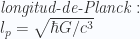 |
 |
| Tiempo | T | 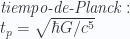 |
![\textit{tiempo-de-Cassini}: \\ t_c= H_0^{-1} =\sqrt{\hbar G /v_0^5} \\ \\ \textit{en-unidades-de-} t_p : \\ t_c = \sqrt[3]{N^5}](https://s0.wp.com/latex.php?latex=%5Ctextit%7Btiempo-de-Cassini%7D%3A++%5C%5C++t_c%3D+H_0%5E%7B-1%7D+%3D%5Csqrt%7B%5Chbar+G+%2Fv_0%5E5%7D++%5C%5C+%5C%5C+%5Ctextit%7Ben-unidades-de-%7D+t_p++%3A+%5C%5C++++t_c+%3D+%5Csqrt%5B3%5D%7BN%5E5%7D+++&bg=fafcff&fg=2a2a2a&s=0&c=20201002) |
| Aceleración | LT -2 |  |
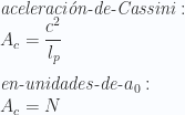 |
| Masa | M |  |
![\textit{masa-de-Planck}: \\ m_p =\sqrt{\hbar c /G} \\ \\ \textit{en-unidades-de-} m_0 : \\ m_p=\sqrt[3]{N}](https://s0.wp.com/latex.php?latex=%5Ctextit%7Bmasa-de-Planck%7D%3A++%5C%5C++m_p+%3D%5Csqrt%7B%5Chbar+c+%2FG%7D++%5C%5C+%5C%5C+%5Ctextit%7Ben-unidades-de-%7D+m_0++%3A+%5C%5C++++m_p%3D%5Csqrt%5B3%5D%7BN%7D+&bg=fafcff&fg=2a2a2a&s=0&c=20201002) |
| Densidad | ML -3 | 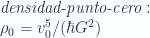 |
![\textit{densidad-de-Planck}: \\ \rho_p=c^5/(\hbar G^2) \\ \\ \textit{en-unidades-de-} \rho_0 : \\ \rho_p=\sqrt[3]{N^{10}}](https://s0.wp.com/latex.php?latex=%5Ctextit%7Bdensidad-de-Planck%7D%3A++%5C%5C++%5Crho_p%3Dc%5E5%2F%28%5Chbar+G%5E2%29+++%5C%5C+%5C%5C+%5Ctextit%7Ben-unidades-de-%7D+%5Crho_0++%3A+%5C%5C+++%5Crho_p%3D%5Csqrt%5B3%5D%7BN%5E%7B10%7D%7D+&bg=fafcff&fg=2a2a2a&s=0&c=20201002) |
| Energ\´ia | ML2T -2 |  |
![\textit{energ\'ia-de-Planck}: \\ E_p=\sqrt{\hbar c^5 /G} \\ \\ \textit{en-unidades-de-} E_0 : \\ E_p=\sqrt[3]{N^5}](https://s0.wp.com/latex.php?latex=%5Ctextit%7Benerg%5C%27ia-de-Planck%7D%3A++%5C%5C++E_p%3D%5Csqrt%7B%5Chbar+c%5E5+%2FG%7D++%5C%5C+%5C%5C+%5Ctextit%7Ben-unidades-de-%7D+E_0++%3A+%5C%5C++E_p%3D%5Csqrt%5B3%5D%7BN%5E5%7D+&bg=fafcff&fg=2a2a2a&s=0&c=20201002) |
| Temperatura | (T) |  |
![\textit{temperatura-de-Planck}: \\ T_p=\sqrt{\hbar c^5 /Gk^2} \\ \\ \textit{en-unidades-de-} T_0 : \\ E_p=\sqrt[3]{N^5}](https://s0.wp.com/latex.php?latex=%5Ctextit%7Btemperatura-de-Planck%7D%3A++%5C%5C++T_p%3D%5Csqrt%7B%5Chbar+c%5E5+%2FGk%5E2%7D++%5C%5C+%5C%5C+%5Ctextit%7Ben-unidades-de-%7D+T_0++%3A+%5C%5C++E_p%3D%5Csqrt%5B3%5D%7BN%5E5%7D+&bg=fafcff&fg=2a2a2a&s=0&c=20201002) |
| Acción | ML 2T -1 |  |
![\textit{constante-de-Cassini}: \\ H_c=\hbar \sqrt{c^5 /v_0^5} \\ \\ \textit{en-unidades-de-} \hbar : \\ H_c =\sqrt[3]{N^5}](https://s0.wp.com/latex.php?latex=%5Ctextit%7Bconstante-de-Cassini%7D%3A++%5C%5C+++H_c%3D%5Chbar+%5Csqrt%7Bc%5E5+%2Fv_0%5E5%7D++%5C%5C+%5C%5C+%5Ctextit%7Ben-unidades-de-%7D+%5Chbar++%3A+%5C%5C+H_c+%3D%5Csqrt%5B3%5D%7BN%5E5%7D++&bg=fafcff&fg=2a2a2a&s=0&c=20201002) |
| Gravedad | ML 3T -2 |  |
 |
| Carga | Q |  |
 |
| Estructura computacional | sin dimensión |  |
 |
| <table cellpadding="10" cellspacing="2" border="1" width="600" style="background-color:#ffffff;text-align:left;color:#000000;font-size:11pt;font-family:times new roman;" > <tr > <td align=center colspan=4 > <strong >COTAS NATURALES del UNIVERSO OBSERVABLE </strong > </td > </tr > <tr > <td align=center > <strong >Magnitud </strong > </td > <td align=center > <strong >Dimensión </strong > </td > <td align=center > <strong >Límite inferior </strong > </td > <td align=center > <strong >Límite superior </strong > </td > </tr ><tr > <td align=center >Velocidad </td > <td align=center > <strong >LT <sup > -1 </sup > </strong > </td > <td align=center valign=top > $latex \textit{velocidad-punto-cero}: \\ v_0 =\sqrt[3]{\hbar G /R_h^2} $ </td > <td align=center valign=top >$latex \textit{(velocidad-de-la-luz)}: \\ c =\sqrt[3]{\hbar G /l_p^2} \\ \\ \textit{en-unidades-de-}v_0 : \\ c =\sqrt[3]{N^2} $ </td > </tr > <tr > <td align=center >Longitud </td > <td align=center > <strong >L </strong > </td > <td align=center valign=top > $latex \textit{longitud-de-Planck}: \\ l_p =\sqrt{\hbar G /c^3} $ </td > <td align=center valign=top >$latex \textit{radio-de-Hubble}: \\ R_h =\sqrt{\hbar G /v_0^3} \\ \\ \textit{en-unidades-de-} l_p : \\ R_h =N $ </td > </tr > <tr > <td align=center >Tiempo </td > <td align=center > <strong >T </strong > </td > <td align=center valign=top > $latex \textit{tiempo-de-Planck}: \\ t_p =\sqrt{\hbar G /c^5} $ </td > <td align=center valign=top >$latex \textit{tiempo-de-Cassini}: \\ t_c= H_0^{-1} =\sqrt{\hbar G /v_0^5} \\ \\ \textit{en-unidades-de-} t_p : \\ t_c = \sqrt[3]{N^5} $ </td > </tr > <tr > <td align=center >Aceleración </td > <td align=center > <strong >LT <sup >-2 </sup > </strong > </td > <td align=center valign=top > $latex \textit{aceleraci\'on-punto-cero}: \\ a_0 = \cfrac{c^2}{R_h} $ </td > <td align=center valign=top >$latex \textit{aceleraci\'on-de-Cassini}: \\ A_c = \cfrac{c^2}{l_p} \\ \\ \textit{en-unidades-de-} a_0 : \\ A_c = N $ </td > </tr > <tr > <td align=center >Masa </td > <td align=center > <strong >M </strong > </td > <td align=center valign=top > $latex \textit{masa-punto-cero}: \\ m_0 =\sqrt{\hbar v_0 /G} $ </td > <td align=center valign=top >$latex \textit{masa-de-Planck}: \\ m_p =\sqrt{\hbar c /G} \\ \\ \textit{en-unidades-de-} m_0 : \\ m_p=\sqrt[3]{N} $ </td > </tr > <tr > <td align=center >Densidad </td > <td align=center > <strong >ML <sup >-3 </sup > </strong > </td > <td align=center valign=top > $latex \textit{densidad-punto-cero}: \\ \rho_0=v_0^5/(\hbar G^2) $ </td > <td align=center valign=top >$latex \textit{densidad-de-Planck}: \\ \rho_p=c^5/(\hbar G^2) \\ \\ \textit{en-unidades-de-} \rho_0 : \\ \rho_p=\sqrt[3]{N^{10}} $ </td > </tr > <tr > <td align=center >Energ\´ia </td > <td align=center > <strong >ML <sup >2 </sup >T <sup >-2 </sup > </strong > </td > <td align=center valign=top > $latex \textit{energ\'ia-punto-cero}: \\ E_0=\sqrt{\hbar v_0^5 /G} $ </td > <td align=center valign=top >$latex \textit{energ\'ia-de-Planck}: \\ E_p=\sqrt{\hbar c^5 /G} \\ \\ \textit{en-unidades-de-} E_0 : \\ E_p=\sqrt[3]{N^5} $ </td > </tr > <tr > <td align=center >Temperatura </td > <td align=center > <strong >(T) </strong > </td > <td align=center valign=top > $latex \textit{temperatura-punto-cero}: \\ T_0=\sqrt{\hbar v_0^5 /Gk^2} $ </td > <td align=center valign=top >$latex \textit{temperatura-de-Planck}: \\ T_p=\sqrt{\hbar c^5 /Gk^2} \\ \\ \textit{en-unidades-de-} T_0 : \\ E_p=\sqrt[3]{N^5} $ </td > </tr > <tr > <td align=center >Acción </td > <td align=center > <strong >ML <sup > 2 </sup >T <sup > -1 </sup > </strong > </td > <td align=center valign=top > $latex \textit{constante-de-Planck-reducida}: \\ \hbar $ </td > <td align=center valign=top >$latex \textit{constante-de-Cassini}: \\ H_c=\hbar \sqrt{c^5 /v_0^5} \\ \\ \textit{en-unidades-de-} \hbar : \\ H_c =\sqrt[3]{N^5} $ </td > </tr > <tr > <td align=center >Gravedad </td > <td align=center > <strong >ML <sup > 3 </sup >T <sup > -2 </sup > </strong > </td > <td align=center valign=top > $latex \textit{gravedad-punto-cero}: \\ G_0=\cfrac{l_p^2v_0^3}{\hbar} $ </td > <td align=center valign=top >$latex \textit{constante-gravitacional}: \\ G=\cfrac{l_p^2c^3}{\hbar} \\ \\ \textit{en-unidades-de-} G_0 : \\ G =N^2 $ </td > </tr > <tr > <td align=center >Carga </td > <td align=center > <strong >Q </strong > </td > <td align=center valign=top > $latex \textit{carga-de-electron}: \\ e_0=\sqrt{\cfrac{4\pi \epsilon_0 \hbar c}{\ln{N}}} $ </td > <td align=center valign=top >$latex \textit{carga-de-Planck}: \\ q_p=\sqrt{4\pi \epsilon_0 \hbar c} \\ \\ \textit{en-unidades-de-} e_0 : \\ q_p =\sqrt{\ln(N)} $ </td > </tr > <tr > <td align=center >Estructura computacional </td > <td align=center > <strong >sin dimensión</strong > </td > <td align=center valign=top > $latex \textit{constante-de-estructura-fina}: \\ \alpha= e_0^2 / (\hbar c 4\pi \epsilon_0) \\\alpha= 1/\ln(N) $ </td > <td align=center valign=top >$latex \textit{capacidad-computacional-universal}: \\ N =\exp(1/\alpha) $ </td > </tr > </table > |
Si tu problema es que no posees un editor de HTML adecuado, te puedo recomendar el mejor editor gratuito WYSIWYG de páginas web, según mi parecer: Es el Amaya versión 11 o superior.
Actualización: Este post ha quedado obsoleto, debido a que el latex de WordPress no admite ya expresiones largas.
Saludos

amarashiki said
¿Te has fijado en cómo ahora no sale tu table con código? Creo que estos días han estado jugando con los temas y los códigos en wordpress… Soy un malpensado, y wordpress.com hace cosas raras con el código LaTeX, además hace unos días cambiaron unas cosas ya ahora no salen en mi tema predeterminado las cosas ordenadas en categorías como antes. ¡Son unos …! No les culpo, al final, piensan como google, facebook o similares…Casi siempre en hacer caja…Aunque me gustaría que wordpress tuviera soporte nativo para LaTeX (vendría genial) y no tener que hacer capturas o burdos malabarismos para evitar usar algunos códigos LaTeX de paquetes especiales de LaTeX. En fin, ya me quejé en wordpress, aunque no creo que hagan caso. Después de todo, ¿cuántos bloggers se centran en el contenido de índole matemática y física mediante ecuaciones? Lo que les interesa son los dibujos o las fotos. Una pena. Supongo que así también cortan el crecimiento del conocimiento en la blogosfera. Una pena.
Saludos.
Albert B. Zotkin said
Es cierto, no sale. Una pena, parece que estos tios van hacia atrás en lugar de progresar. Por ejemplo, si quiero poner el lagrangiano completo del SM, ahora tengo que trocear el código en varias partes, para que cada parte no sea demasiado larga,
O sea una chapuza. Una pena.
amarashiki said
¿Has reeditado tú la tabla de LaTeX o ha reaparecido sola?
Albert B. Zotkin said
La he reeditado yo, jeje, pero esta vez con latex externo a wordpress. Usé el latex renderer de numberempire.com. Si no has usado nunca un latex externo a wordpress (hay muchos), te explico un poco como funciona. Para el caso del latex de numberempire.com, si quieres escribir, por ejemplo, la función Zeta de Riemann, debes poner el código para insertar imagen así: <img src=”http://www.numberempire.com/equation.render?\zeta(s)=\sum_{n=1}^\infty \frac{1}{n^s}”>. Si quieres que aparezca algún texto sobre la imagen latex cuando paras el cursor del ratón sobre ella, debes escribir <img title=”este texto aparece cuando situas el cursor sobre la imagen” src=”http://www.numberempire.com/equation.render?\zeta(s)=\sum_{n=1}^\infty \frac{1}{n^s}”>
Saludos
amarashiki said
¿Sabes algo de MathJaX? Estoy preparando el nuevo dominio (espero tenerlo listo en el cumpleaños de mi blog, el mes que viene), pero dudo de si es mejor instalar la app de soporte de LaTeX o bien probar con MathJaX en el mismo mejor que con LaTeX, pero no sé si MathJaX permitiría personalización de código LaTeX, ¿sabes de alguien que lo haya usado? He preguntado en twitter, pero nadie me ha dado una respuesta sensata…De hecho no he recibio ni una sola respuesta…YO me suelo fiar poco de los sistemas de renderización porque al final, pueden fallar o perder soporte…Y yo conozco unos cuantos que de un tiempo a esta parte desaparecieron…No sé, a ver qué hago, porque ¡wordpress me está haciendo perder demasiado tiempo en cuestiones de lenguage y técnicas de soporte TeX que no esperaba a estas alturas!
Albert B. Zotkin said
Si, claro, lo sé todo. Es muy fácil usar MathJaX, pero es muy limitado (por ejemplo, no tiene la versatilidad de los programas de edición de documentos TeX) . Si vas a tener un servidor que aloje tu blog, es una opción decente poner MathJax (tus propias copias de las librerias instaladas en tu servidor web), pero siempre teniendo en mente que no podrás hacer mucho más de lo que hacías con el LaTeX de WordPress. En cuanto a lo que dices de que tienes dudas de si te permitiría personalizar código LaTex, no sé a qué te refieres. El propio código LaTex te permite ya dar algo de formato (personalizar), con sus comandos, a sus objetos.
Albert B. Zotkin said
He estado viendo algunas cosas más sobre MathJax, sobre todo opiniones de usuarios. En mi opinión existen dos serios inconvenientes para usar MathJax. El primero, y más importante, es que ralentiza brutalmente la carga de una página web que posea algo para ser procesado con MathJax. Mira lo que decía el año pasado Luboš Motl en su blog al respecto, Testing Mathjax. De todas formas, hasta hoy, Luboš Motl sigue usando MathJax en su blog, quizás porque él no abusa mucho en sus posts del LaTeX, y por eso piensa que compensa seguir usándolo. El segundo inconveniente que le veo a MathJax es que si no has instalado correctamente algunas extensiones, entonces algunos comandos LaTeX no son reconocidos, y eso limita bastante las posibilidades de escribir matemáticas con MathJax si no eres un experto en la materia.
Saludos
LOG#074. Dual units. « The Spectrum of Riemannium said
[…] I have never seen such an idea published before, so I translated to English the table he posted here in Spanish […]
LOG#074. Dual units. | The Spectrum Of Riemannium said
[…] I have never seen such an idea published before, so I translated to English the table he posted here in Spanish […]